The techniques of Fourier analysis that you've learned in this are remarkable for a few reasons, but one reason is that it sets up a correspondence between understanding real space and Fourier space.

Let's take the very simple example of the square wave from Example 12.1 where we found that $$f(x) \sim \sum_{k=1}^\infty b_k \sin(\lambda_k x)$$ and $\lambda_k = k$ and $b_k = 4/(k\pi)$ if $k$ is odd (otherwise it is zero). I'll use $k$ here for the index because it is more typical when this topic comes up.

We can imagine two spaces: the $(x, f(x))$ space where the original signal exists, and the Fourier space-$(k, b_k)$. We will refer to $(k, b_k)$ as Fourier space or the Fourier spectra or the spectrum. You can think of these words as simply referring to the collection of wavenumbers $k$ and amplitudes.

What is sound? Here is a picture.

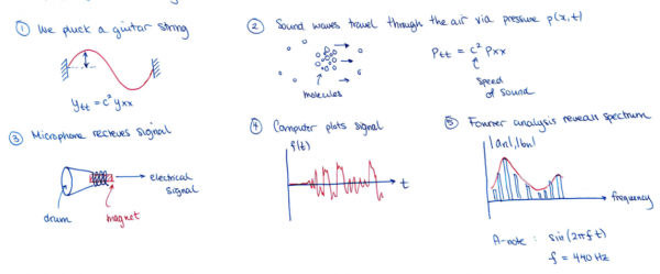
When you learn about Fourier series, you can either work with functions $f(x)$ or functions $f(t)$. Since we're dealing with sound, we want to work with $f(t)$ and consider the pressure vibrations that are detected by our microphone in time. Let's sort out the terminology. We write out a basic sine wave like this: $$f(t) = \sin(2\pi f t) \qquad 0 \leq t \leq t_f.$$

The quantity $f$ is called the frequency of the wave. It has units of $s^{-1}$ (1-over-seconds) and we call this unit a Hertz, Hz. Notice the wavelength is $2\pi/(2\pi f) = 1/f$. When referring to time, we say “period” instead of “wavelength”.

So for example, if $f = 100Hz$, the period is 1/100 s, so that in one second, the signal completes 100 cycles.

Now a digital representation of the note will not be continuous in time but instead we need to record the note at a certain sampling frequency $F_s$. In other words, in the length of time $t_f$, we record the signal in steps of $\Delta t = 1/F_s$.

For example, Matlab's default sample rate for their built-in sound function is $F_s = 10^{13} = 8192$ Hz. Let's show how we make a digital sound and then output it to our speakers.

Fs = 2^(13); T = 5; t = 0:(1/Fs):T;
f = sin(2*pi*440*t); sound(f, Fs);

The 440Hz signal is what is known as an A note. Musicians often use this note to tune or calibrate their instruments. On a violin, which has four strings, the highest string plays an E note when it is tuned properly, and this has a frequency of 639.3 Hz.

The last thing I want to show you today is how a computer stores the information of a signal in terms of a Fourier series. Rather than store information about sines and cosines separately, it is more compact to work with complex-valued functions and store the information together.

Matlab uses the fft command to calculate the Fourier series of a signal (technically the discrete Fourier transform). I will not explain it in detail at this point. What you have to understand is that you can put a vector into fft, but to plot the Fourier amplitudes, you need to rearrange the output in a funny way.

N = length(f);
yhat = fft(f);
A = abs(yhat)/N;
K = (Fs/2)*(1:ceil(N/2))/ceil(N/2);
A = A(1:ceil(N/2));
plot(K, A)

(We noticed during the lecture that the above code is flawed by 1 element, as it indicates a peak frequency of 441Hz instead of 440Hz! I believe this is because you have to 'dump' one of the vector components).